Usage

Installation

The hughes2d package dependencies are managed using uv (see [uv](https://docs.astral.sh/uv/)). If uv is installed, you can install the hughes2d package and its dependencies by typing:

git clone --depth 1 https://github.com/TheoRGirard/hughes2d
cd hughes2d
uv sync

The core of the hughes2d package only depends on numpy and triangle. However, there are several optional dependencies (see below).

Plots

If you want to use plot functionnalities you should also add matplotlib or plotly:

uv add matplotlib

or install the extras:

uv sync --extra plot

Note

If both matplotlib and plotly, the default preference is set to plotly.

File format handling

If you want to import .dxf, .msh or FreeFEM mesh files, you should include the file-format extra:

uv sync --extra file-formats

You can also include all the extras:

Without uv

If you don’t have uv installed, you can see a list of the dependencies in the _pyproject.toml_ file (or below).

hughes2d v0.1.0
├── numpy v2.2.2
├── triangle v20250106
│   └── numpy v2.2.2
├── ezdxf v1.3.5 (extra: file-formats)
│   ├── fonttools v4.55.8
│   ├── numpy v2.2.2
│   ├── pyparsing v3.2.1
│   └── typing-extensions v4.12.2
├── meshio v5.3.5 (extra: file-formats)
│   ├── numpy v2.2.2
│   └── rich v13.9.4
│       ├── markdown-it-py v3.0.0
│       │   └── mdurl v0.1.2
│       └── pygments v2.19.1
├── matplotlib v3.10.0 (extra: plot)
│   ├── contourpy v1.3.1
│   │   └── numpy v2.2.2
│   ├── cycler v0.12.1
│   ├── fonttools v4.55.8
│   ├── kiwisolver v1.4.8
│   ├── numpy v2.2.2
│   ├── packaging v24.2
│   ├── pillow v11.1.0
│   ├── pyparsing v3.2.1
│   └── python-dateutil v2.9.0.post0
│       └── six v1.17.0
├── plotly v6.0.0 (extra: plot)
│   ├── narwhals v1.24.1
│   └── packaging v24.2
├── pyqt6 v6.8.1 (extra: plot)
│   ├── pyqt6-qt6 v6.8.2
│   └── pyqt6-sip v13.10.0

You can either install the dependencies with pip:

git clone https://github.com/TheoRGirard/hughes2d
cd hughes2d
pip install -r requirements.txt
pip install -e

or install the dependencies manually.

Getting started

You can find a file named _getting_started.py_ in /examples/00-getting_started. We rewrite below the content of this file.

from pathlib import Path

from hughes2d import CellValueMap, Mesh, NonConvexDomain, PedestrianSolver

file_path = str(Path(__file__).parent / "gettingStartedSimu")

#Construction of the domain--------------------------------
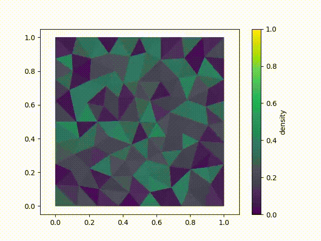
MyDomain = NonConvexDomain([[0,0],[0,1],[1,1],[1,0]])
MyDomain.add_exits([[[1,0],[1,1]]])

#construction of the Mesh--------------------------------------
MyMesh = Mesh()
MyMesh.generate_mesh_from_domain(MyDomain, 0.01)
MyMesh.save_to_json(file_path)


#Construction of the initial datum ---------------------------------------
MyMap = CellValueMap(MyMesh)
MyMap.generate_random()

#Setting the options for the simulation-----------------------------------------
opt = {
    "model" : "hughes",
    "filename" : file_path,
    "save" : True,
    "verbose" : False,
        }

#Creating the solver and computing---------------------------------------------------
Solver = PedestrianSolver(MyMesh, 0.01, initial_density = MyMap, options=opt)
Solver.compute_until_empty(100)

#Converting the data to a mp4 video------------------------------------------
try:
    import matplotlib.pyplot as plt
except ImportError:
    plt = None

if plt:
    from hughes2d import Plotter
    Plotter.convert_to_mp4(file_path, limits=[[0,1],[0,1]])

Compiling and running this code should create 3 .csv files, 1 .json file.

Additionally, if matplotlib is installed, the last part of this script should produce a .mp4 file. The .mp4 file should look like the video below:

Basic usage

We cover below the basic usages of the hughes2d package. The content of this section approximately matches with the examples present in the /examples/ folder.

Note:: Check out the examples (https://github.com/TheoRGirard/hughes2d/tree/main/examples) on the repository for short demonstrations of further functionnalities. Check out the Geometry reference for a complete reference of the classes and methods of the package.

Constructing a domain

The NonConvexDomain object is used to define a domain. Here a domain is defined by a set of walls, exits. Walls and exits are pretty explicit (note however that a domain should necessarily contain at least one exit for the simulation to compute properly).

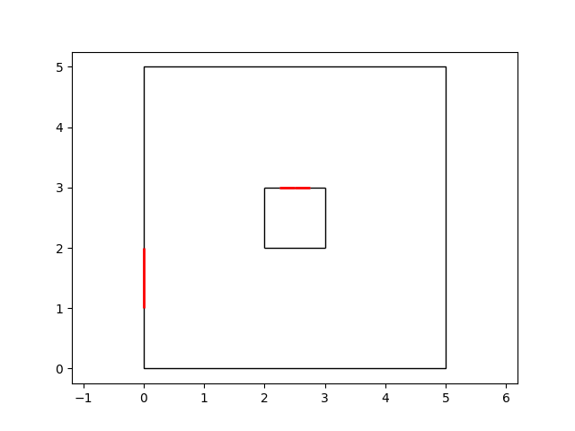
Here is an example of the script used to define the following domain:

from hughes2d import NonConvexDomain

big_square_points = [[0,0],[5,0],[5,5],[0,5]]
small_square_points = [[2,2],[2,3],[3,3],[3,2]]

Innerwall = [[1,1],[1,4]]

#Domain construction -----------------------------
Domain1 = NonConvexDomain(big_square_points)
Domain1.add_wall(small_square_points, cycle=True)
Domain1.add_wall(Innerwall, cycle=False)

When cycling is set to True, the space inside the convex hull of small_square_points is excluded from the domain. On the contrary, the wall defined by Innerwall is of 0 thickness.

Remember that we need to set up exits as well:

Exit1 = [[0,1],[0,2]]
Exit2 = [[2.25,3],[2.75,3]]
Exit3 = [[5,1],[5,2]]

Domain1.add_exit(Exit1) #One at a time
Domain1.add_exits([Exit2,Exit3]) #Or multiple

Then we can visualize the domain using

Domain1.show()

If no preference is set, plotly will be used. Plotly will open an instance of your preferred navigator in order to show the domain on a localhost port. If you prefer matplotlib, use:

Domain1.show(preference="matplotlib")

Generating a mesh

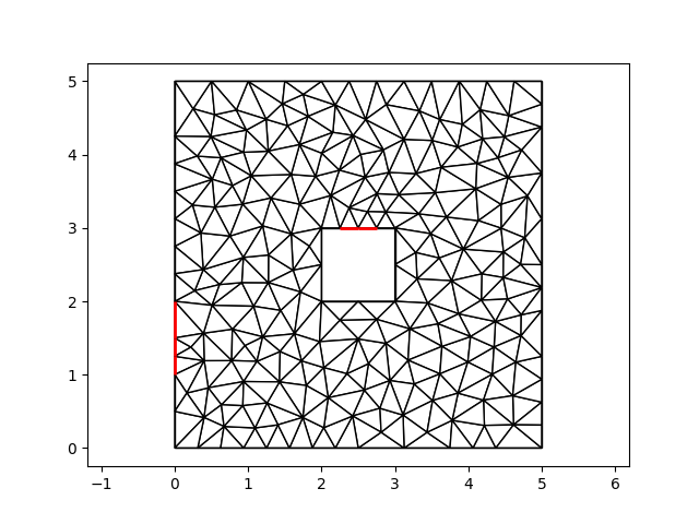
If you have defined a NonConvexDomain object, you can simply generate a Mesh using the domain. Here is an example:

MyMesh = Mesh()
MyMesh.generate_mesh_from_domain(Domain1, dx=0.1, da=20)

The dx corresponds to the maximal area of a triangle in the mesh and da corresponds to the minimal angle of a triangle in the mesh.

Note

Be careful: the generation time is inversely proportional to dx. Also the generation time explodes as da goes to 45.

You can visualize the mesh by using MyMesh.show() and obtain something like:

You can now pass to the definition of an initial datum step in order to use the Mesh for a simulation. We recommand saving your mesh as a .json file in order to save computation time, instead of generating a mesh for each execution.

from pathlib import Path

MyMesh.save_to_json(str(Path(__file__).parent / "square"))

Produces a “square_mesh.json” file. You can load it using:

MyMesh2 = Mesh()
MyMesh2.load_from_json(str(Path(__file__).parent / "square_mesh.json"))

Importing a mesh

Instead of generating a mesh from a NonConvexDomain you can also import an external mesh. The available options at the moment are:

Mesh.import_from_lists: an import from explicit python lists.
Mesh.import_mesh_from_msh: an import from a GMSH-defined .msh file.
Mesh.import_mesh_from_msh_free_fem: an import from a FreeFEM defined .msh file.

We defer to the [complete reference](https://hughes2d.readthedocs.io/en/latest/reference.html) of the Mesh object in the documentation for further details.

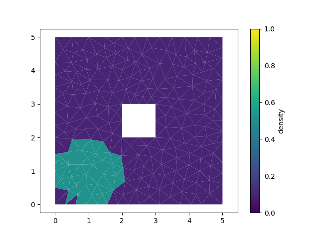
Defining the initial datum

Once you have a Mesh object defined, you first need to define the initial datum for your simulation:

::

from hughes2d import CellValueMap

MyMap = CellValueMap(MyMesh) MyMap.generate_random()

Here the initial density of pedestrian is random (CellValueMap.generate_random()). You can also use the method CellValueMap.set_constant() to… set the density equal to a constant everywhere in the domain. Or alternatively, use

MyMap.set_constant_circle(center=[1,1], radius = 1, value = 0.7)

in order to get something like:

You can also add and multiply two CellValueMap objects together. And you can visualize the datum using CellValueMap.show(). We defer to the object reference for more details.

Launching the simulation

Now all that’s left is to launch the simulation on the mesh MyMesh with the initial datum MyMap. This is pretty straigth-forward:

from hughes2d import PedestrianSolver

opt = { "model" : "hughes" }
Solver = PedestrianSolver(MyMesh, dt = 0.01, initial_density = MyMap, options = opt)
Solver.compute_until_empty(max_frames = 1000)

Here we launch a simulation of Hughes’ model (the opt dictionary) with a time step of 0.01 (be careful with taking big time step values, the simulation might crash). We compute the solution until the domain is empty (or we hit the maximal number of frame, here 1000). If you set opt[“verbose”]=True more informations will be displayed in the console. If you set opt[“save”]=True the data from the simulation will be stored in data files named as opt[“filename”]. There are many more options to play with in the options dictionary, see the section dedicated to it below.

Plotting the results

There are many ways of visualizing the simulation results once the computations have ended. First, since each time step corresponds to a CellValueMap object you can just plot it along the simulation:

for _ in range(10):
    Solver.compute_step() # Computes one time step
    Solver.lwr_solver.show_density(t=0)

You can also create a .mp4 file from the data files obtained with the simulation (see the 08-Plot_methods examples):

from pathlib import Path

import hughes2d.Plotter

filename = "path/to/datafile_base_name"
hughes2d.Plotter.convert_to_mp4(filename)

The opt dictionary

We detail here the different options available in the opt dictionary passed as a parameter to the PedestrianSolver object:

{
  "model" : "hughes", #(string) switch between different models among { "hughes", "colombo-garavello" , "constantDirectionField" }
  "filename" = "path/to/file_basename", #(string) filename serving as a basename for the saved files
  "save" : True, #(boolean) saving or not the computed data
  "verbose" : True, #(boolean) printing messages in the console
  "lwrSolver" : {
            "convexFlux" : True, #(boolean) if the flux function is convex, setting this to true switch from dichotomy to explicit computations
            "anNum" : "dichotomy", #(string) chose the method of computation if not explicit between : dichotomy, Newton (not available for the moment...)
            "method" : "midVector", #(string) method of resolution of the edge discontinuous flux : between 'tmap' (transmission maps) and 'midVector' (continuous godunov scheme with an averaged vector between the two triangles)
            "ApproximationThreshold" : 0.0001,
            }, #(float) the approximation threshold for the computed values
  "eikoSolver" : {
            "constrained" : True, #(boolean) if set to True, the considered gradient for the Fast marching algorythm must stay inside the triangle from which it is computed.
            "NarrowBandDepth" : 2, #(int) thickness (in number of neighbouring degree) of the narrow band.
            },
}

Licence

The Hughes2d package is free software: you can redistribute it and/or modify it under the terms of the GNU General Public License as published by the Free Software Foundation, either version 3 of the License, or (at your option) any later version.

The Hughes2d package is distributed in the hope that it will be useful, but WITHOUT ANY WARRANTY; without even the implied warranty of MERCHANTABILITY or FITNESS FOR A PARTICULAR PURPOSE. See the GNU General Public License for more details.

You should have received a copy of the GNU General Public License along with the Hughes2d package. If not, see <https://www.gnu.org/licenses/>.