Mathematics

Macroscopic pedestrian models

The mathematical models for pedestrian crowds can be catyegorized in three main categories.

The microscopic models use a huge number of agents interacting with each other to model a crowd of pedestrian. This type of model often relies on the use of a system coupling many Ordinary Differential Equation (ODE).
The mesoscopic models deal with an infinite number of agents characterized by an artificial parameter. This type of model mainly consists in kinetic partial differential equations and uses the formalism of statistic physics.
The macroscopic models deal with a density of pedestrian instead of agents. This type of model relies on the use of Partial Differential Equation (PDE) which are often close to the PDEs found in fluid dynamics.

The present python package focuses on the numerical approximation of solutions to Hughes’ model (introduced in [Hug02] ) which is one of most studied the macroscopic models.

Hughes’ model

Note

The introduction to Hughes’ model below is quoted from the introduction of Chapter 2 of [Gir25]. It is recommanded reading it there as more detail are included.

In [Hug02], Hughes proposed a mathematical model for the two-dimensional dynamics of pedestrian crowds. The model consists in a system of two equations set on a bounded domain $\Omega \subset \mathbb{R}^2$. The first PDE is a vector-directed scalar conservation law with discontinuous flux. The second is an Eikonal equation with discontinuous source term.

The scalar conservation law

The first equation models the flow of a density $\rho$. To be more precise $\rho(t,x)$ represents the density of pedestrian at time $t$ and location $x$. It is bounded between $0$ and a given $\rho_{max} >0$. We assume that the pedestrian move with the speed of agents $v(t,x)$ at time $t$ and location $x$ following a unitary direction field $\vec{V}(t,x) \in \mathcal{S}_1$. Then, if we write the conservation of the mass on pedestrian on each subdomain of $\Omega$, we end up with the following scalar conservation law:

\[\partial_t \rho + \mathbf{div}(\vec{V}(t,x) v(t,x) \rho(t,x)) = 0.\]

In Hughes’ model, we assume that the speed of agents $v(t,x)$ at time $t$ and location $x$ only depends on the density $\rho(t,x)$ and that this speed is decreasing with respect to the density. Then, in the following we will denote the speed by $v(\rho(t,x))$ where $v$ is a decreasing function defined on $[0,\rho_{max}]$ such that

\[v(0)=: v_{\max} \textrm{ and } v(\rho_{max})= 0.\]

A classical example of such a speed function is $v(\rho) = v_{max}\frac{\rho_{max}-\rho}{\rho_{max}}$. This corresponds to the very classical Lighthill-Whitham-Richards (LWR) model for traffic flows (see [LW55], [Ric56]).

The Eikonal equation

The second equation of the model characterizes the unitary direction field $\vec{V}(t,x)$ depending on the density $\rho$ in the whole domain. We assume that the pedestrians want to minimize their exit time while also trying to avoid high density regions. In order to model this situation, we use an optimal control problem. We suppose that the density $\rho(\cdot) \in \mathcal{C}^1(\bar \Omega)$ stays constant in time (this assumption is quite controversial). Let $x \in \Omega$. For any $\alpha(\cdot) \in \mathcal{C}^1((0,+\infty),\mathcal{S}_1)$, we say that $X^\alpha_x(\cdot)$ is a trajectory controlled by $\alpha$ starting at $x$ if $X$ is a solution to the Cauchy problem:

\[\begin{split}\left\lbrace \begin{matrix} \dot{X}^\alpha_x(s) = \alpha(s)v(\rho(t,X^\alpha_x(s))) \\ X^\alpha_x(0) = x \end{matrix}\right.\end{split}\]

For any $x \in \Omega$, we denote by $\mathcal{A}_x = \{ X^\alpha_x, \alpha \in \mathcal{C}^1((0,+\infty),\mathcal{S}_1) \}$ the set of all controlled trajectories starting at $x$. We define $\phi(x)$ as the minimal exit time starting at location $x$, that is to say:

\[\phi(x) = \inf_{X \in \mathcal{A}_x} \int_0^{+\infty} \mathbb{1}_{\Omega}(X(t)) \textrm{d} t.\]

In Hughes’ model, we also take into account the discomfort caused by being surrounded by a high density crowd. In order to model this discomfort, we introduce an increasing function $g(\rho)$ with respect to the density $\rho$. The function $g(\rho)$ can be interpreted as a running cost we are paying along a trajectory $X$ for being in high density regions. Then, the previous equation becomes:

\[\phi(x) = \inf_{X \in \mathcal{A}_x} \int_0^{+\infty} \mathbb{1}_{\Omega}(X(t))g(\rho(X(t))) \textrm{d} t.\]

A very classical result of the theory of viscosity solution for Hamilton-Jacobi-Bellman (HJB) equations is that solving the optimal control problem above is in fact equivalent to solving the Eikonal equation:

\[\begin{split}\left\lbrace \begin{matrix} |\nabla \phi (x) | = \frac{g(\rho(x))}{v(\rho(x))} && x \in \Omega\\ \phi(x) = 0 && x \in \partial\Omega \end{matrix}\right.\end{split}\]

We now claim that the direction field $\vec{V}(t,x)$ should be the unitary descending gradient of $\phi$. If we suppose that there exists $X^*_x$ an optimal trajectory, i.e. $\phi(x) = \int_0^{+\infty} \mathbb{1}_\Omega(X^*_x(t))g(\rho(X^*_x(t)))\textrm{d} t$, then we have

\[\vec{V}(t,x) = \dot{X}^*_x(0) = -\frac{\nabla \phi(x)}{|\nabla \phi(x)|}.\]

The Hughes model definition

Then the complete Hughes’ model introduced in [Hug02] was the following:

\[\begin{split}\left\lbrace \begin{matrix} \partial_t \rho + \mathbf{div}(\vec{V}(t,x) v(t,x) \rho(t,x)) = 0 \\ \vec{V}(t,x) = -\frac{\nabla \phi}{|\nabla \phi|} \\ |\nabla \phi (t,x) | = \frac{g(\rho(t,x))}{v(\rho(t,x))} && x \in \Omega\\ \phi(t,x) = 0 && x \in \partial\Omega. \end{matrix}\right.\end{split}\]

Note

Here, we chose to present the Hughes’ model without any wall around or inside the domain for consiness’ sake. Keep in mind that for a domain with walls and exits, both equations should be solved with mixed boundary condition i.e. Neumann non-crossing conditions on the walls and Dirichlet free-exit boundary conditions on the exits.

For a deep overview of the mathematical results regarding Hughes’ model we defer to [AADF+23].

Model of Colombo-Garavello-Lécureux-Mercier

In [CGLM11], the authors introduced an alternative model for pedestrian flows.

In this model, the agents chose the shortest path to the exits without taking the density into account. This corresponds to the Eikonal equation with constant source term:

\[|\nabla u (x)| = 1.\]

Then the vector field prescribing the direction of the agents $\vec{V}(x)$ is a combination between the direction of the shortest path $\frac{-\nabla u}{|\nabla u|}$ and a non-local deviation operator $\mathcal{I}[\rho](x)$. In [CGLM11], the authors propose the a definition for the non-local operator: let $\eta_r(\cdot)$ be a mollifier compactly supported in the ball of radius $r > 0$; then we define:

\[\mathcal{I}[\rho](x) = - \epsilon \frac{\nabla \rho * \eta_r}{\sqrt{1+|\nabla \rho * \eta_r|^2}}.\]

Note:: The operator above depends on two real parameters: the radius r and the amount of deviation epsilon. These parameters corresponds to the parameters of the dictionary CGparameters in the python package.

In the present package, we denote by the Colombo-Garavello-Lecureux-Mercier model the following (slightly modified) system:

\[\begin{split}\left\{ \begin{matrix} \partial_t \rho + \mathbf{div}(\vec{V}(t,x) v(t,x) \rho(t,x)) = 0 \\ |\nabla \phi (t,x) | = 1 \\ \vec{\nu}(x) = - \frac{\nabla \phi}{|\nabla \phi|} \\ \mathcal{I}[\rho](x) = - \epsilon \frac{\nabla \rho * \eta_r}{\sqrt{1+|\nablla \rho * \eta_r|^2}}\\ \vec{V}(t,x) = \frac{ \vec{\nu}(x) + \mathcal{I}[\rho](x) }{| \vec{\nu}(x) + \mathcal{I}[\rho](x) |} \end{matrix}\right.\end{split}\]

This model is also featured in the present python package.

Numerical schemes

Note

The presentation of the numerical schemes below is quoted from the introduction of Section 4.5.1 of [Gir25]. It is recommanded reading it there as more detail are included.

The numerical scheme we propose consists in two coupled algorithms, each of them approximating, at one time step, one of the equations of Hughes’ model ($\rho$ or $V=\nabla \phi$, respectively) given the solution of the other equation.

Mesh definition

Let $T>0$. Let $J \in \mathbb{N}^*$. We discretize the interval $[0,T]$ as $J + 1$ time steps and we set:

\[\Delta t := \frac{T}{J}, \;\; t^j := j\Delta t.\]

We suppose that $\Omega$ is a polygonal domain. Let $\Delta x > 0$.

Let $\underline{\textrm{$\triangle$}}, |\triangle| > 0$, we denote $\Delta x := (\underline{\textrm{$\triangle$}}, |\triangle|)$. We consider a triangular mesh defined by a set of open triangles $M_\Delta := (\mathcal{T}_n)_{1 \leq n \leq N}$ such that

for all $1\leq n \leq N$, the area of the triangle $\mathcal{T}_n$ denoted by $|\mathcal{T}_n|$ satisfies $0 < |\mathcal{T}_n| \leq |\triangle|$.
for all $1\leq n \leq N$, if we denote $\mathcal{T}_n = A_nB_nC_n$ then $\max \{ |A_n B_n|, |A_n C_n|, |C_n B_n|\} \leq \underline{\textrm{$\triangle$}}$.
for any $1 \leq i,j \leq N$, we have $\mathcal{T}_i \bigcap \mathcal{T}_j = \emptyset$ and

\[\begin{split}\bar{\mathcal{T}}_i \bigcap \bar{\mathcal{T}}_j \neq \emptyset \Rightarrow &\textrm{ upon reparametrization of the points of the triangle }\\ &\textrm{either } \bar{\mathcal{T}}_i \bigcap \bar{\mathcal{T}}_j = \{A_i\} = \{ A_j \},\\ &\textrm{or } \bar{\mathcal{T}}_i \bigcap \bar{\mathcal{T}}_j = [A_iB_i] = [ A_j B_j].\end{split}\]

$\bigcup_n \bar{\mathcal{T}}_n = \bar\Omega$.

We use the following notations:

the set of all the vertices is denoted by $V_\Delta$.
we say that two points of $V_\Delta$ are neighbours if there exists a triangle in $M_\Delta$ such that both points are vertices of the triangle.
for any $P \in V_\Delta$, we denote by $\mathcal{V}(P)$ the set of neighbours of $P$.
we denote by $T_\Delta(P)$ the set of all the triangles of $M_\Delta$ having $P$ as one of its vertices.

We also denote $N := \mathbf{Card}(M_{\Delta x})$ i.e. $M_{\Delta x} = (\mathcal{T}_n)_{1\leq n \leq N}$.

General overview of the scheme

Let the initial datum $\rho_0$ be lower semi-continuous (so that the Eikonal equation is well posed, see [Gir25]). We discretize $\rho_0$ by defining, for any $n \in \mathbb{N}$,

\[\rho^0_n = \inf_{x \in \mathcal{T}_n} \rho_0(x), \;\; \rho^0_\Delta(x) := \sum_{1\leq n \leq N} \mathbb{1}_{\mathcal{T}_n}(x) \rho^0_n.\]

Let $\rho_\Delta : \bar\Omega \rightarrow \mathbb{R}$ be constant on the triangles of $M_{\Delta x}$ i.e. $\forall n \in [\![ 1, N ]\!], \; \exists \rho_n \in \mathbb{R},$ such that $\forall x \in \mathcal{T}_n, \;\; \rho_\Delta(x) = \rho_n$. Then, we define the lower semi-continuous envelope of $\rho_\Delta$ by:

\[\begin{split}\rho_{\Delta*}(x) := \min_{\begin{matrix}n \in [\![ 1, N ]\!], \\ \textrm{ s.t. } x \in \overline{\textrm{$\mathcal{T}_n$}}\end{matrix}} \rho_n.\end{split}\]

Then, we will apply the following procedure iteratively for any $j \in [\![ 0 , J ]\!]$.

We compute a numerical approximation $\phi^j_\Delta$ of the solution to the eikonal equation

\[\begin{split}\left\{ \begin{matrix} |\nabla \phi| = c((\rho^j_{\Delta})_*) &x \in \bar\Omega \setminus \mathcal{E}\\ \phi(x) = 0 &x \in \mathcal{E}.\end{matrix}\right.\end{split}\]

We use either a $\mathbf{FMT}$, a $\mathbf{FME}$ (see [Gir25]) or a third algorithm (detailled below) named the $\mathbf{FMTC}$ algorithm.

We compute $V^j_\Delta$ corresponding to the unit vector opposite to the gradient of $\phi_\Delta^j$ on each triangle $(\mathcal{T}_n)_{1\leq n \leq N}$. In order to compute $V^j_\Delta$, we denote $\mathcal{T}_n = ABC$. As $\phi_\Delta^j$ is affine on $ABC$, the gradient is constant and, for any $n \in [\![ 1, N ]\!]$, we set:

\[V_n^j := \frac{1}{\mathcal{H}_{ABC}(\phi(A),\phi(B),\phi(C))}\times \frac{(\phi(B) - \phi(A))\vec{AB}^\bot - (\phi(C) - \phi(A))\vec{AC}^\bot}{\det(\vec{AC},\vec{AB})}.\]

See [Gir25] for more details about this formula. We define $V^j_\Delta$ by:

\[V^j_\Delta(x) := \sum_{1\leq n\leq N} \mathbb{1}_{\mathcal{T}_n}(x) V_n^j.\]

We compute a numerical approximation $\rho^{j+1}_\Delta$ of $\rho(\Delta t,\cdot)$ where $\rho$ is the solution to

\[\begin{split}\left\{ \begin{matrix} \rho_t + \div \left[ f(\rho) V^j_\Delta \right] = 0 &(t,x) \in (0,\Delta t) \times \Omega\\ \rho = 0 &x \in \mathcal{E}\\ f(\rho)(V^j_\Delta \cdot \vec{n}) = 0 &x \in \mathcal{W} \\ \rho(0,x) = \rho^j_\Delta(x). \end{matrix}\right.\end{split}\]

We use a finite volume scheme on $M_\Delta$ in order to approximate $\rho$. We propose two different computations for the flux on the edges of the mesh, namely the discontinuous flux method and the weighted flux method. See below for details about the finite volume scheme and the different methods.

The finite volume scheme for the SCL

In this paragraph, we present the explicit finite volume scheme we will use to compute $(\rho^{j+1}_n)_{1\leq n \leq N}$ knowing $(\rho^{j}_n)_{1\leq n \leq N}$ and $(V^{j}_n)_{1\leq n \leq N}$. We suppose that the maximal density $\rho_{max}$ equals $1$ i.e. we suppose that the flux function $f$ is Lipschitz, concave and such that $f(0) = f(1) = 0$ and that $\rho_0 \in [0,1]$. We introduce a few additional notations.

Let $M \in \mathbb{N}$ be the number of distinct edges in the mesh $M_\Delta$. We denote by $E_\Delta := (e_m)_{1\leq m \leq M}$ the set of all the edges of the triangles of $M_\Delta$.
For any $n \in [\![ 1, N ]\!]$, we denote by $E_n$ the set of all the edges of $\mathcal{T}_n$.
For any $m \in [\![ 1, M ]\!]$, we denote by $\mathcal E^m$ the set of all triangles of $M_\Delta$ that admit $e_m$ as one of its edges. Notice that $\mathbf{Card}(\mathcal{E}^m) \in \{1,2\}$.
For any $m \in [\![ 1, M ]\!]$, we denote by $|e_m|$ the geometrical length of the edge $|e_m|$.
For any $m \in [\![ 1, M ]\!]$, for any $\mathcal{T} \in \mathcal{E}^m$, we denote by $\vec{n}_m(\mathcal{T})$ the unit normal vector to $e_m$ that is pointing outward of $\mathcal{T}$.
For any $\mathcal{T} \in M_\Delta$ we denote $\rho^j_{\mathcal{T}} := \rho^j_n$ where $\mathcal{T}_n = \mathcal{T}$. Analogously, we denote $V^j_{\mathcal{T}} := V^j_n$ where $\mathcal{T}_n = \mathcal{T}$.

We also recall that, for any $f:\mathbb{R} \rightarrow \mathbb{R}$, for any $a,b \in \mathbb{R}$, the Godunov numerical flux is defined by:

\[\begin{split}\mathbf{God}_f(a,b) := \left\{ \begin{matrix} \min_{c \in [a,b]} f(c) &\textrm{if } a \leq b \\ \max_{c \in [b,a]} f(c) &\textrm{if } b < a. \end{matrix} \right.\end{split}\]

The finite volume scheme corresponds to the following algorithm for any fixed $j \in [\![ 0, J ]\!]$.

For any $m \in [\![ 1, M ]\!]$, we denote

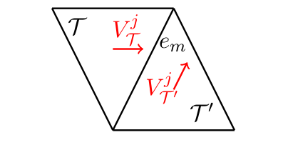
\[\mathcal{E}^m = \{ \mathcal{T} \} \textrm{ if } \mathbf{Card}(\mathcal{E}^m) =1, \mathcal{E}^m = \{ \mathcal{T}, \mathcal{T}' \} \textrm{ if } \mathbf{Card}(\mathcal{E}^m) =2.\]

We want to compute the flux $f^j_m(\mathcal{T})$ crossing the edge $e_m$ coming from $\mathcal T$. We distinguish between the two following cases.

If $\mathbf{Card}(\mathcal E^m) = 2$, we propose two different methods to compute $f^j_m(\mathcal{T})$.

The discontinuous flux method: we use a dichotomy method to find $k \in [0,1]$ such that:

\[\mathbf{God}_{V^j_{\mathcal{T} } \cdot \vec{n}_m(\mathcal{T})f}(\rho^j_{\mathcal T},k)-\mathbf{God}_{V^j_{\mathcal{T'} } \cdot \vec{n}_m(\mathcal{T})f}(k,\rho^j_{\mathcal T'}) = 0.\]

Then we set:

\[f^j_m(\mathcal{T}) := \mathbf{God}_{V^j_{\mathcal{T}} \cdot \vec{n}_m(\mathcal{T})f}(\rho^j_{\mathcal T},k).\]

The textbf{weighted flux} method: first, if $V^j{\mathcal{T}} \rho^j_{\mathcal{T}} + V^j{\mathcal{T'}} \rho^j_{\mathcal{T'}} \neq \vec{0}$, we define

\[\vec{v}_m(\mathcal{T}) := \frac{V^j{\mathcal{T}} \rho^j_{\mathcal{T}} + V^j{\mathcal{T'}} \rho^j_{\mathcal{T'}}}{\left|V^j{\mathcal{T}} \rho^j_{\mathcal{T}} + V^j{\mathcal{T'}} \rho^j_{\mathcal{T'}}\right|}.\]

If $V^j{\mathcal{T}} \rho^j_{\mathcal{T}} + V^j{\mathcal{T'}} \rho^j_{\mathcal{T'}} = \vec{0}$, we set $\vec{v}_m(\mathcal{T}) = \vec{0}$. Then we set:

\[f^j_m(\mathcal{T}) := \mathbf{God}_{\vec{v}_m(\mathcal{T})\cdot \vec{n}_m(\mathcal{T}) f}(\rho^j_{\mathcal T},\rho^j_{\mathcal T'}).\]

Else if $\mathbf{Card}(\mathcal E^m) = 1$, we have that $e_m \in \partial \Omega$. Then, once again we distinguish between two cases.

If $e_m \in \mathcal{E}$, we set:

\[f^j_m(\mathcal{T}) := \mathbf{God}_{V^j_{\mathcal{T}} \cdot \vec{n}_m(\mathcal{T}) f}(\rho^j_{\mathcal T},0).\]

Else if $e_m \in \mathcal{W}$, we set:

\[f^j_m(\mathcal{T}) := 0.\]

For any $n \in [\![ 1, N ]\!]$, we set

\[\rho^{j+1}_n := \rho^{j}_n - \frac{\Delta t}{|\mathcal{T}_n|} \sum_{e_m \in E_n} f_m^j(\mathcal{T}_n) |e_m|.\]

Note

The discontinuous flux method correspond to the algorithm detailled in cite{AbrahamPreprint}. Heuristically, we are solving the SCL while assuming there is a discontinuity of $V^j_\Delta$ at each edge of $E_\Delta$. If $V_\Delta^j$ is constant across the edge $e_m$ then the discontinuous flux method is equivalent to setting

\[f^j_m(\mathcal{T}) := \mathbf{God}_{V^j_{\mathcal{T}} \cdot \vec{n}_m(\mathcal{T})f}(\rho^j_{\mathcal T},\rho^j_{\mathcal T'}),\]

which corresponds exactly to the classical Godunov numerical flux in the continuous case. The discontinuous flux method correponds exactly to the use of the identity $k \mapsto k$ “transmission map”, in the terminology of cite{CancesAndreianov2015}.

Note

The weighted flux method corresponds to the following procedure: we define $\vec{v}_m(\mathcal{T})$ as a weighted mean of the two vectors $V^j_{\mathcal{T}}$ and $V^j_{\mathcal{T}'}$; then eqref{eq:defMidVecFlux} corresponds to the classical Godunov numerical flux as if we had $V^j_{\mathcal{T}}=V^j_{\mathcal{T}'}=\vec{v}_m(\mathcal{T})$. The heuristics for this method comes from the following situation.

Notice that, here, we have:

\[V^j_{\mathcal{T}'}\cdot \vec{n}_m(\mathcal{T}) = 0.\]

Then, if we use the discontinuous flux method, for any $\rho_{\mathcal{T}}^j, \rho_{\mathcal{T}'}^j \in [0,1]$ we have $f_m^j(\mathcal{T}) = 0$. Then there is no flux exiting the cell $\mathcal{T}$ even if $\rho_{\mathcal{T}'}^j = 0$. Heuristically, this means that the agents of cell $\mathcal{T}$ are prevented from moving in the direction $V^j_{\mathcal{T}}$ because the “phantom” agents of cell $\mathcal{T}'$ (since the cell is almost empty) should move in the incompatible direction $V^j_{\mathcal{T}'}$. This heuristic is our inspiration to consider, as a practical alternative, the weighted flux method. Indeed, if we use the weighted flux method, if $\rho_{\mathcal{T}}^j \gg \rho_{\mathcal{T}'}^j$ then we have that $\vec{v}_m(\mathcal{T}) \simeq V_{\mathcal{T}}^j$. Then

\[f_m^j \simeq \max_{c \in [\rho_{\mathcal{T}'}^j,\rho_{\mathcal{T}}^j]} f(c) \;\; V_{\mathcal{T}}^j \cdot \vec{n}_m(\mathcal{T}) \gg 0.\]

This represents a kind of “majority-rule” where the direction of the high density cells prevails over the direction of the low density cells.

Warning

Even if we do not provide any proof of convergence for the above finite volume scheme in [Gir25], we can still derive the CFL condition that guarantees the monotonicity and the stability of the scheme. Here the CFL takes the following form:

\[\Delta t \leq \frac{\underline{|\triangle|}}{3\underline{\textrm{$\triangle$}}Lip_f},\]

where $\underline{|\triangle|}$ denotes the minimal area of a triangle in $M_\Delta$. The numerical experiments with the present package must be done under the above CFL condition !

Scheme for the eikonal equation: the FMTC algorithm

In this paragraph, we fix $j \in [\![ 0, j ]\!]$. Then, for any $n \in [\![ 0, N]\!]$, we set:

\[c_n := c(\rho^j_n).\]

We define $\phi_\Delta : V_\Delta \rightarrow \mathbb{R}^+$ as the solution of the $\mathbf{FMTC}$ numerical scheme. Let $P^0 = V_\Delta \bigcap E$. We set $\phi_\Delta(P) = 0$ for any $P \in P^0$. For any $m \in \mathbb{N}$, we introduce the following iterative $\mathbf{FMTC}$ procedure, using the conceptual framework of Fast Marching algorithms where $P^m$ denotes the given set of “frozen” vertices of the mesh at step $m$.

We compute the set of neighbours among which we will choose the next vertex (or vertices) to freeze (named the “narrow band”):

\[NB^m = \left\{ P \in V_\Delta \setminus P^m \textrm{ s.t. } \exists Q \in P^m, P \in \mathcal{V}(Q) \right\}.\]

If $NB^m = \emptyset$, the algorithm is terminated.
Else, for any $A \in NB^m$, we compute $\mathcal{V}_A$ as described below.

We consider $(\mathcal{T}_k)_{1\leq k \leq K}$ the set of all triangles of $M_\Delta$ such that $A$ is one of the vertices of the triangle and at least one other vertex of the triangle is in $P^m$. Denote by $ABC$ the triangle $\mathcal{T}_k$.

For each $k$ we compute $V^k_A$ distinguishing between three cases.

If only $B$ (resp. only $C$) is in $P_m$, then $V_A^k = \phi_\Delta(B) + |AB| c_k$ (resp. $V_A^k = \phi_\Delta(C) + |AC| c_k$ ).

If $B$ and $C$ are both in $P^m$, we suppose, up to renaming the vertices, that $\phi_\Delta(B) \leq \phi_\Delta(C)$. We denote $V_B := \phi_\Delta(B)$ and $V_C = \phi_\Delta(C)$. Then we set $V_A^k = \tilde{V}_A$ where $\tilde{V}_A$ is defined by eqref{eq:defTildeVa} i.e.

\[\begin{split}V_A^k := \left\{ \begin{matrix} &V_B + F|AB| \qquad\qquad\qquad\qquad \textrm{ if } c_k\; \vec{AB}\cdot\vec{BC} +(V_C -V_B)|AB| >0 \\ \\ &V_C + F|AC| \qquad\qquad\qquad\qquad \textrm{ if } c_k\; \vec{AC}\cdot\vec{BC} +(V_C -V_B)|AC| <0 \\ \\ &V_B + \frac{\vec{AB}\cdot\vec{CB}}{BC^2}(V_C-V_B) + |\det(\vec{AB},\vec{CB})| \frac{\sqrt{(c_k)^2 BC^2 - (V_C-V_B)^2}}{BC^2} \qquad \textrm{ else. }\end{matrix}\right.\end{split}\]

Then we set

\[\mathcal{V}_A := \min_k \{ V_A^k \}.\]

We freeze the point $P = \mathbf{argmin}_{A \in NB^m} \mathcal{V}_A$ i.e. $P^{m+1} = P^m \cup \{ P \}$. We set $\phi_\Delta(P) = \mathcal{V}_P$. If multiple points satisfy $\phi_\Delta(P) = \mathcal{V}_P$, we freeze all these points. We loop back to step 1.

In the following, we denote by $\phi_\Delta$ the unique function of $W^{1,\infty}(\bar\Omega)$ that is affine on each triangle and $\phi_\Delta(P)$ is given by the above algorythm for any $P \in V_\Delta$.

Bibliography

[AADF+23]

Debora Amadori, Boris Andreianov, Marco Di Francesco, Simone Fagioli, Théo Girard, Paola Goatin, Peter Markowich, Jan F. Pietschmann, Massimiliano D. Rosini, Giovanni Russo, Graziano Stivaletta, and Marie-Therese Wolfram. The mathematical theory of Hughes’ model : a survey of results. In Crowd Dynamics, Volume 4 : Analytics and Human Factors in Crowd Modeling, Modeling and Simulation in Science, Engineering and Technology. Springer, 2023.

[CGLM11] (1,2)

Rinaldo M. Colombo, Mauro Garavello, and Magali Lécureux-Mercier. A class of nonlocal models for pedestrian traffic. Mathematical Models and Methods in Applied Sciences, 22:1150023, 2011.

[Gir25] (1,2,3,4,5,6)

Théo Girard. On singular Hamilton-Jacobi-Bellman and scalar conservation laws encountered in pedestrian models. Mathematics [math]. Université de Tours, 2025.

[Hug02] (1,2,3)

Roger L. Hughes. A continuum theory for the flow of pedestrians. Transportation Research Part B-methodological, 36:507–535, 2002.

[LW55]

Michael J Lighthill and Gerald Beresford Whitham. On kinematic waves. II. A theory of traffic flow on long crowded roads. Proceedings of the Royal Society of London A: Mathematical, Physical and Engineering Sciences, 229(1178):317–345, 1955.

[Ric56]

Paul I Richards. Shock waves on the highway. Operations research, 4(1):42–51, 1956.